Data Processing
You must write a report using Word or LibreOffice and place it in the folder u:\DocumentsDevoir\Nom_du_Prof.
Ви повинні підготувати звіт у Word або LibreOffice та зберегти його в папці u:\DocumentsDevoir\Nom_du_Prof.
Vous devrez réaliser un compte rendu avec Word ou Libreoffice que vous déposerez dans le dossier
u:\DocumentsDevoir\Nom_du_Prof\.
- Question 3.1 (from pix exam)
• Open the file vente (click here)
As shown in this video: click here
• Add a new row for product 5 with a quantity sold of 32 and a unit price of 15 euros
• Calculate how much revenue each product generated by completing the “sold” column
• Calculate the total revenue generated by all products
• Add a grid around the table and make the headers and the table border thicker
• Відкрити файл vente (натисніть тут)
Як показано в цьому відео: натисніть тут
• Додати рядок для продукту 5 із кількістю проданих одиниць 32 та ціною 15 євро за штуку
• Обчислити, скільки приніс продаж кожного продукту, заповнивши стовпець «продано»
• Обчислити, скільки в цілому приніс продаж усіх продуктів
• Обвести таблицю сіткою та зробити заголовки й рамку таблиці товстішими
- Ouvrir le fichier vente ( cliquez-ici)
Comme montré dans cette vidéo: cliquez-ici
- Ajouter une ligne produit 5 avec un quantité de produit vendu de 32 et un prix unitaire de 15 euros
- Calculer combien a rapporté la vente de chaque produit en complétant la colonne à vendu
- Calculer combien a rapporté la vente de l'ensemble des produits
- Entourer le tableau d'une grille et épaissir les titres et le tour du tableau
- Question 3.2
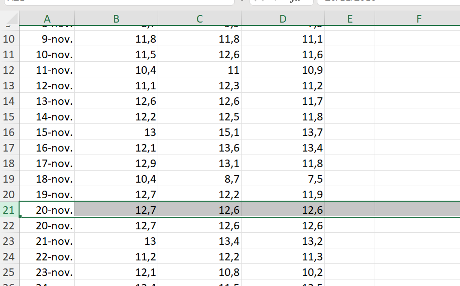
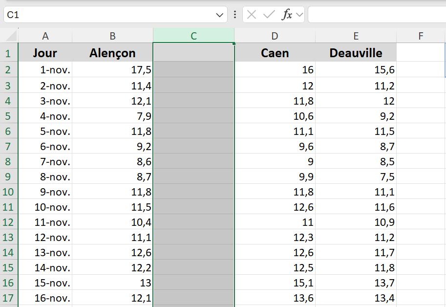
Odile has prepared a file containing the maximum temperatures for November 2016 in 4 cities.
In the Bilan sheet:
• The row for November 20 is duplicated. Delete one of the two rows.
• Insert a column between Alençon and Caen, and copy into it the data from the Bellengreville sheet.
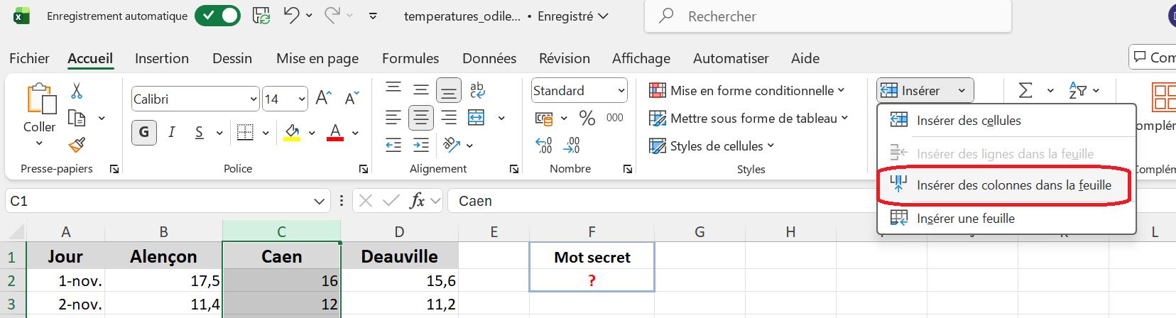
What secret word appears in cell G2?
Follow the steps below to complete the exercise:
- Open Odile’s file (click here)
- Left‑click on row number 21 to select row 21

Suivre la démarche ci-dessous pour réaliser l'exercice
- Ouvrir le fichier d'Odile ( cliquez-ici)
- cliquer gauche sur le numéro 21 pour sélectionner la ligne 21

Виконайте наступні кроки, щоб завершити вправу:
• Відкрийте файл Оділь (натисніть тут)
• Клацніть лівою кнопкою миші на номері рядка 21, щоб вибрати рядок 21
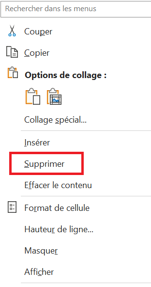
- Right‑click on row 21 to display the dialog box (fig. 1) with the Delete option, or click Delete in the Home menu (fig. 2). In both cases, row 21 is deleted
- cliquer droit sur la ligne 21 pour faire apparaître la boite de dialogue (fig 1) avec l'option Supprimer ou cliquer sur Supprimer du menu Accueil (fig2) dans les deux cas la ligne 21 est supprimée. 
 ou
ou 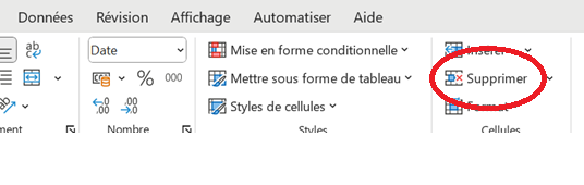
fig1 fig2
- Left‑click on the letter C to select the Caen column.
- cliquer gauche sur le C pour sélectionner la colonne Caen:
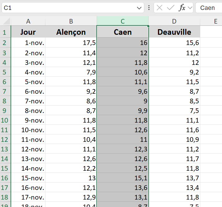
- Left‑click the Insert button in the Home menu, then choose Insert Sheet Columns (shown in red below).
- cliquer gauche sur le bouton insérer du menu Accueil puis choisir Insérer des colonnes dans la feuille ( en rouge ci-dessous):

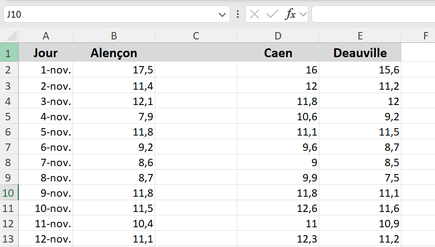
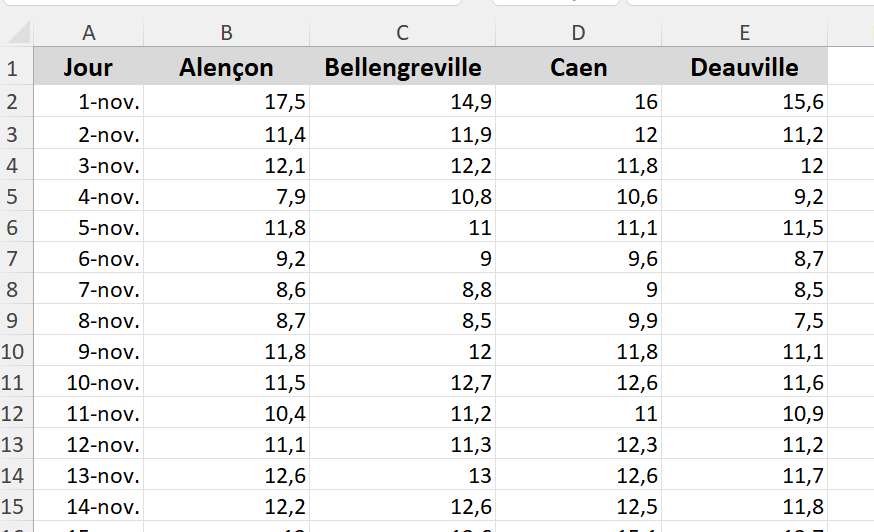
Result:
Résultat:
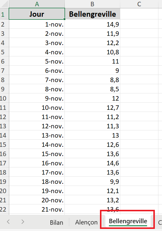
- Select the Bellengreville sheet by left‑clicking on the Bellengreville tab at the bottom of the Excel window (highlighted in red below).
- Sélectionner la feuille Bellengreville en cliquant gauche sur le nom de l'onglet Bellengreville en bas de la feuille excel encadré en rouge ci-dessous:
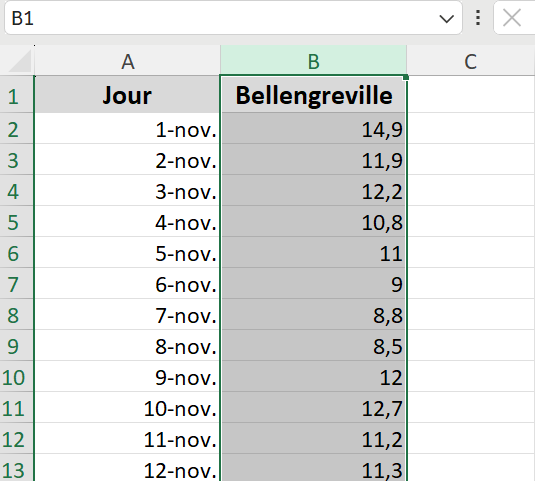
- Left‑click on the letter B to select the Bellengreville column, then click the Copy button in the Home menu (outlined in red below).
- Cliquer gauche sur le B pour sélectionner la colonne Bellengreville puis sur le bouton Copier du menu Accueil (entouré en rouge ci-dessous):

- Select the Bilan sheet by left‑clicking on the Bilan tab at the bottom of the Excel window. Then left‑click on the letter C to select the column, and left‑click the Paste button in the Home menu to paste the Bellengreville data into column C.
- Sélectionner la feuille Bilan en cliquant gauche sur le nom de l'onglet Bilan en bas de la feuille excel. Puis cliquer gauche sur le C pour sélectionner la colonne, cliquer gauche sur le bouton Coller du menu Accueil pour coller les données de Bellengreville dans la colonne C
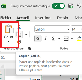
Result:
Résultat:
- Take a screenshot of the word that appears in cell G2.
- Faire une capture d'écran du mot qui apparaît dans la cellule G2

- Question 3.3
- In the file (click-here) , which postal code appears on line 8
У файлі який ((натисніть тут)) поштовий індекс зазначено в рядку 8?
- Dans le fichier ( cliquez-ici) quel code postal figure sur la ligne 8 ?
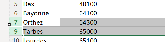
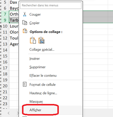
Row 8 is hidden. Select rows 7 and 9, which surround the hidden row 8, right‑click, then choose Unhide.
La ligne 8 est masquée, sélectionner les lignes 7 et 9 qui entourent la ligne 8 masquée, faire un clic-droit puis
sélectionner Afficher

- Chart creation
In this section, you will explore a few concepts related to plotting graphs with Excel.
Dans cette partie vous allez voir quelques notions autour du tracé de graphes avec Excel.
У цій частині ви ознайомитеся з кількома поняттями, пов’язаними з побудовою графіків в Excel.
- Question 3.4
plotting graph with scatter plots
- Open the file graphiqueXY (click here)
- Watch the video on XY curve plotting if needed (click here)
tracé de courbes avec nuages de points
- Ouvrir le fichier graphiqueXY ( cliquez-ici)
- Regarder si nécessaire la video sur le tracé de courbe XY: cliquez-ici
побудова кривих за допомогою точкових діаграм
• Відкрити файл graphiqueXY (натисніть тут)
• За потреби переглянути відео про побудову XY‑кривої (натисніть тут)
As shown in the video:
- Select the X and Y data. Plot the curve x = f(y) using a smoothed scatter plot with markers, add the title of the X‑axis and the Y‑axis.
- What is the name in French of the type of curve obtained?
Comme montré dans la vidéo:
- Sélectionner les données X et Y. Tracer la courbe x=f(y) avec un nuage de points courbe lissée et marqueur, ajouter le titre de l'axe X et celui de l'axe Y, quelle est le nom du type de courbe obtenu ?

- Select the Z and T data, create a scatter plot, and note the number that appears.
- Sélectionner les données Z et T , demander un nuage de points, quelle est le nombre qui s'affiche? 
- Question 3.5
• Open the graphique file (click here)
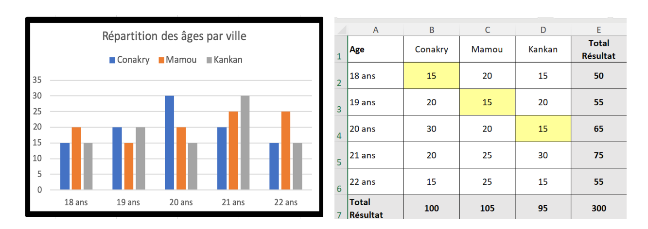
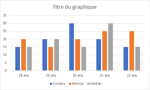
• We want to create the chart shown on the left below using the data shown on the right below.
- Ouvrir le fichier graphique ( cliquez-ici)
- On veut réaliser le graphique ci-dessous à gauche à partir des données ci-dessous à droite:
- Відкрити файл graphique (натисніть тут)
- Потрібно побудувати діаграму, зображену нижче ліворуч, використовуючи дані, наведені нижче праворуч.
Méthod:
here are data
voici les données:
Ось дані.
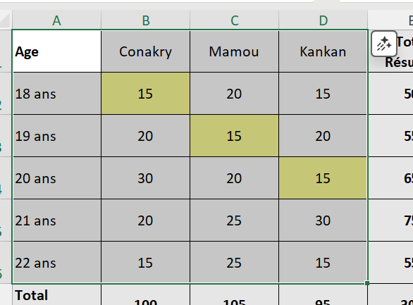
- Select the cells from A1 to D6.
- Sélectionner les cellules de A1 à D6,
- Виділіть комірки від A1 до D6.
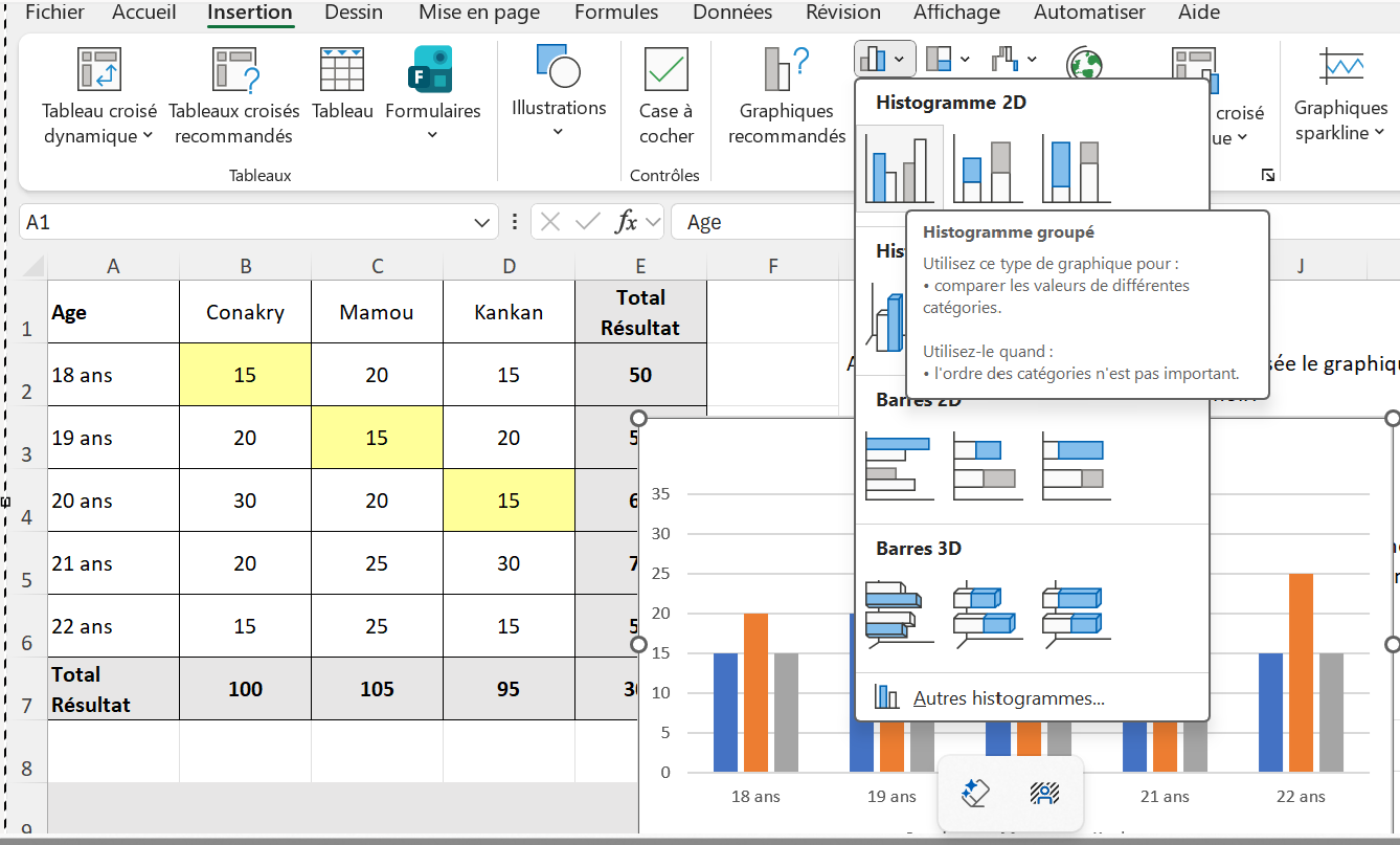
Then click on Insert a 2D Histogram.
puis cliquer sur Insertion d'un Historigramme 2D
потім натисніть Вставити гістограму 2D.
You get:
Vous obtenez:
Compared to what we want to obtain in the final result, you need to add the chart title and move the legend to the top:
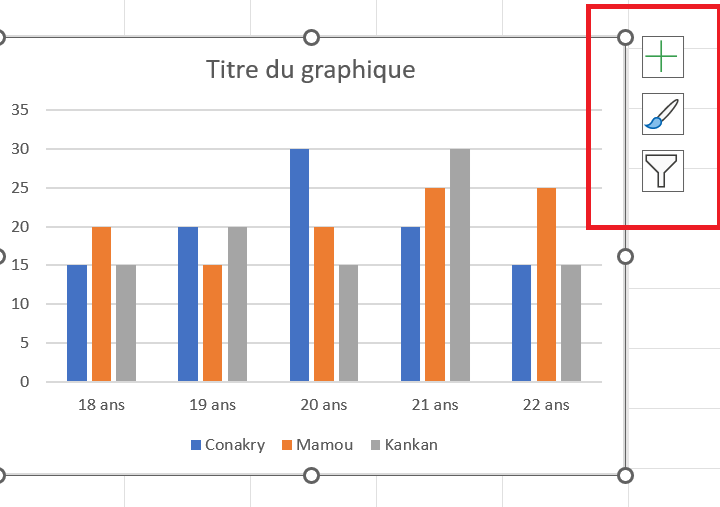
- Move your chart into the grey area (located on the left, below the data table). When the chart is selected, three buttons appear (outlined in red below). These buttons allow you to reconfigure the chart in different ways
Par rapport à ce que l'on doit obtenir au final, il faut ajouter le titre du graphique et déplacer la légende en haut:
- Déplacer votre graphique en zone grisée ( située à gauche en dessous du tableau de données), lorsque le graphe est sélectionné il apparaît les 3 boutons (encadrés en rouge ci-dessous), ces boutons permettent de reconfigurer différemment le graphique:
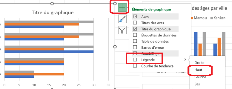
- Click the + button, then click Legend, then click the arrow to the right of Legend (see the screenshot below). Select Top; the legend will then be placed at the top.
- Cliquer sur le bouton + puis sur légende puis sur la flèche à droite de Légende ( voir la capture ci-dessous), sélectionner en Haut, la légende se retrouve placée en haut:
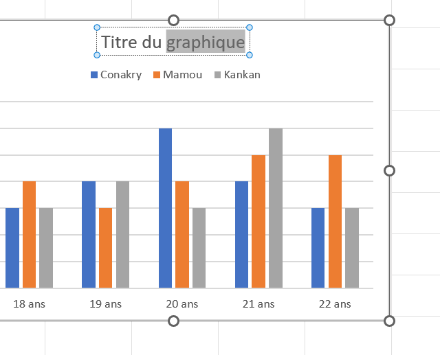
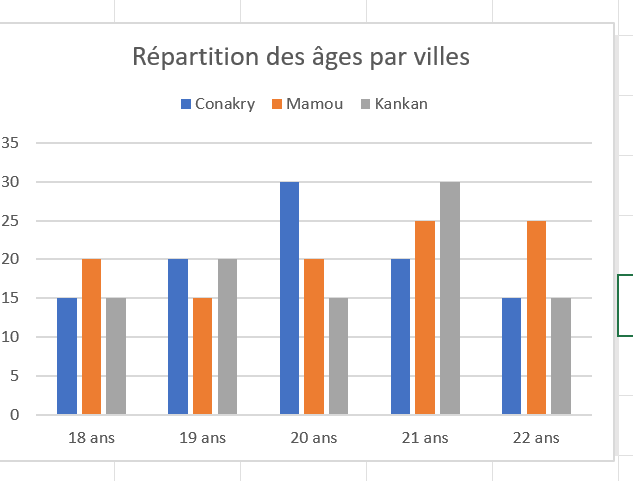
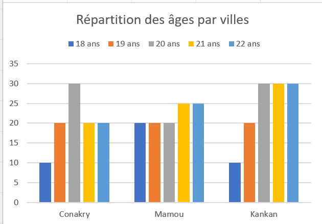
- Double‑click on Chart Title (on the left below) and replace the text with Distribution of ages by city. You should obtain the view shown on the right below.
- Double-cliquer sur Titre du graphique ( à gauche ci-dessous) et remplacer le texte par Répartition des âges par villes, vous devez obtenir la vue à droite ci-dessous:
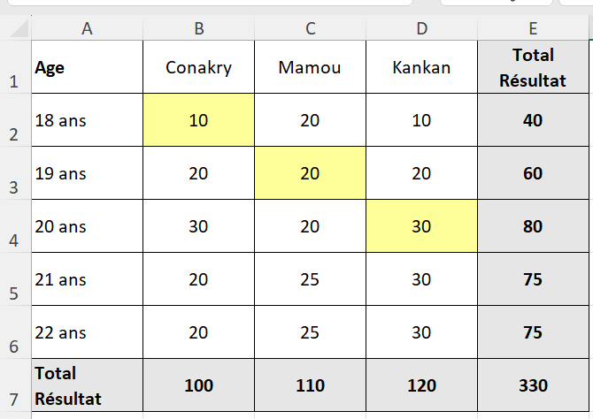
- Change the values in the table by entering 10 in B2, 20 in C3, and 30 in D4, result:
- Modifier les valeurs du tableau en mettant 10 en B2, 20 en C3 et 30 en D4, résultat:
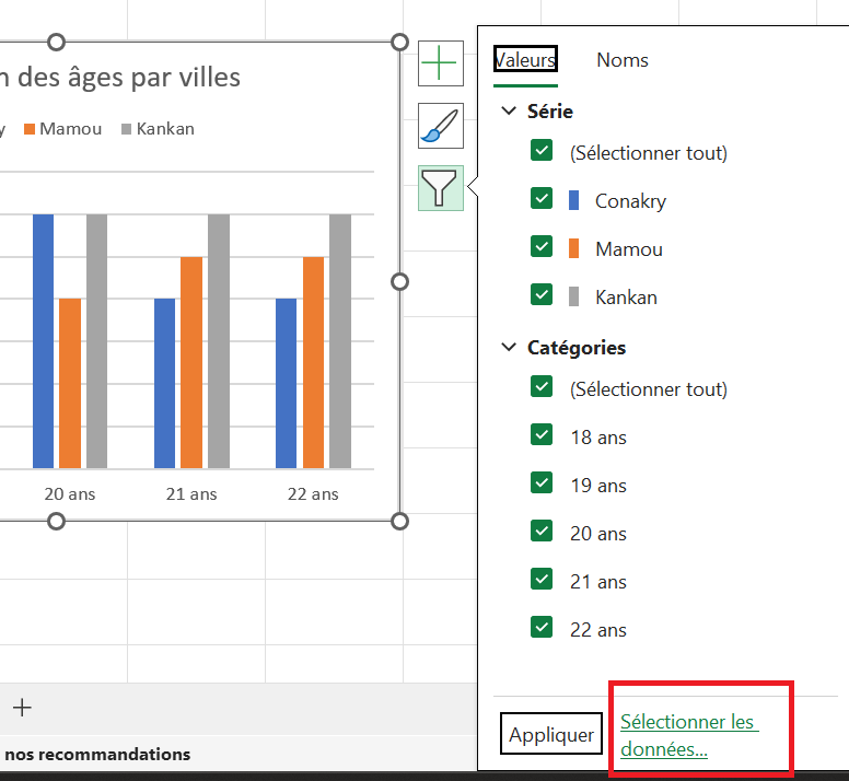
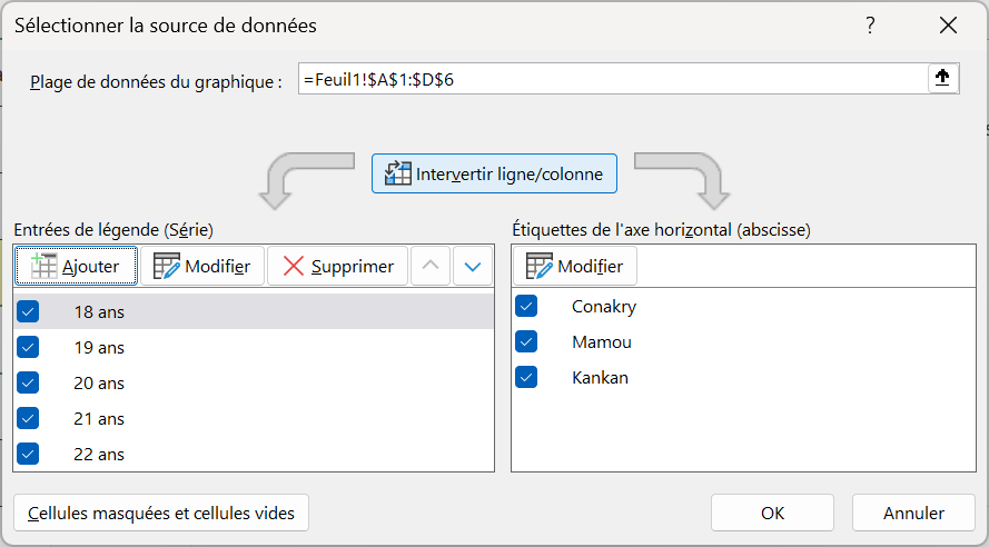
- Switch the orientation of the data series (rows ↔ columns). To do this, click the funnel‑shaped button (on the left below), then click Select Data (outlined in red below). The dialog box shown on the right below will appear; click the Switch Row/Column button (in blue on the right below).
- Intervertir l'orientation des séries de données ( lignes-colonnes), pour ça cliquer le bouton en forme d’entonnoir ( à gauche ci-dessous) puis cliquer sur Sélectionner des données ( encadré en rouge ci-dessous), la boite de dialogue ci-dessous à droite apparaît, cliquer sur le bouton Intervertir ligne/colonne ( en bleu ci-dessous à droite) :

You get:
Vous obtenez:
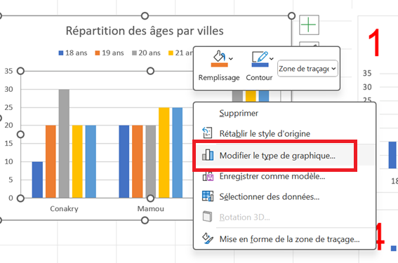
- Right‑click the chart and choose Change Chart Type (shown on the left below), then select a Bar chart type (shown on the right below).
- Cliquer droit sur le graphique et choisir Modifier le type de graphique ( ci-dessous à gauche) , Choisir un type Barres ( ci-dessous à droite) :

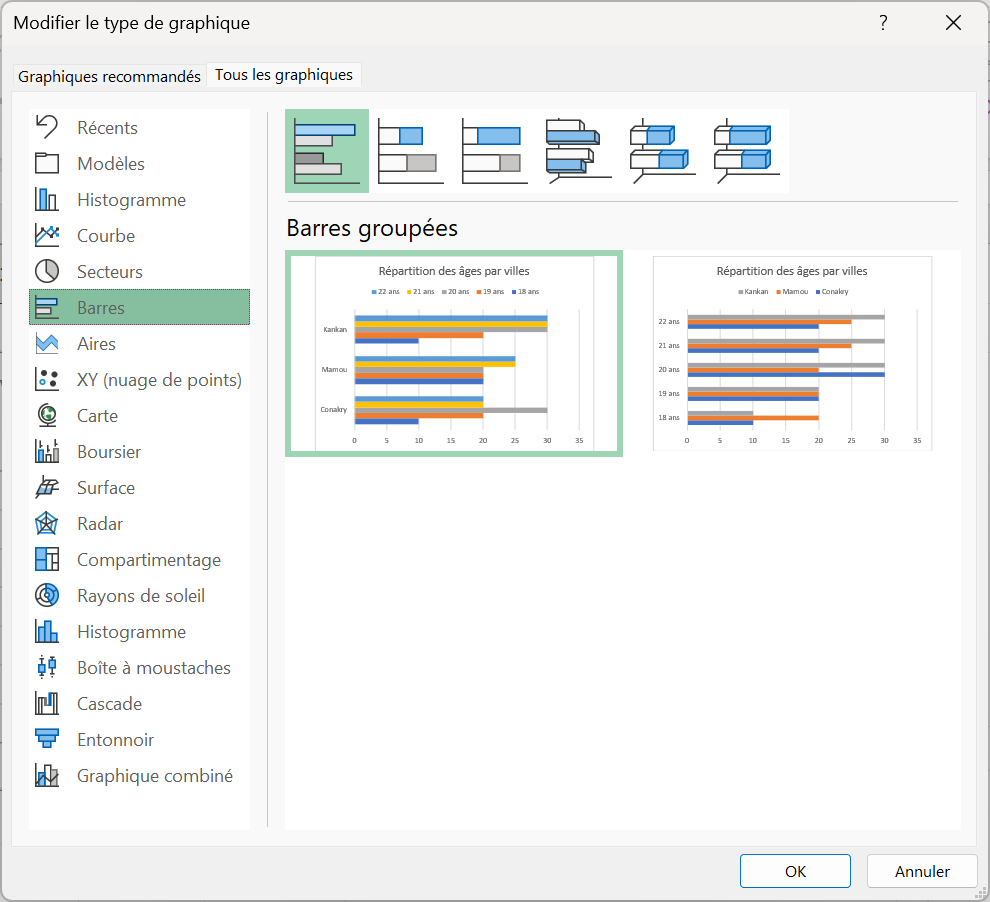
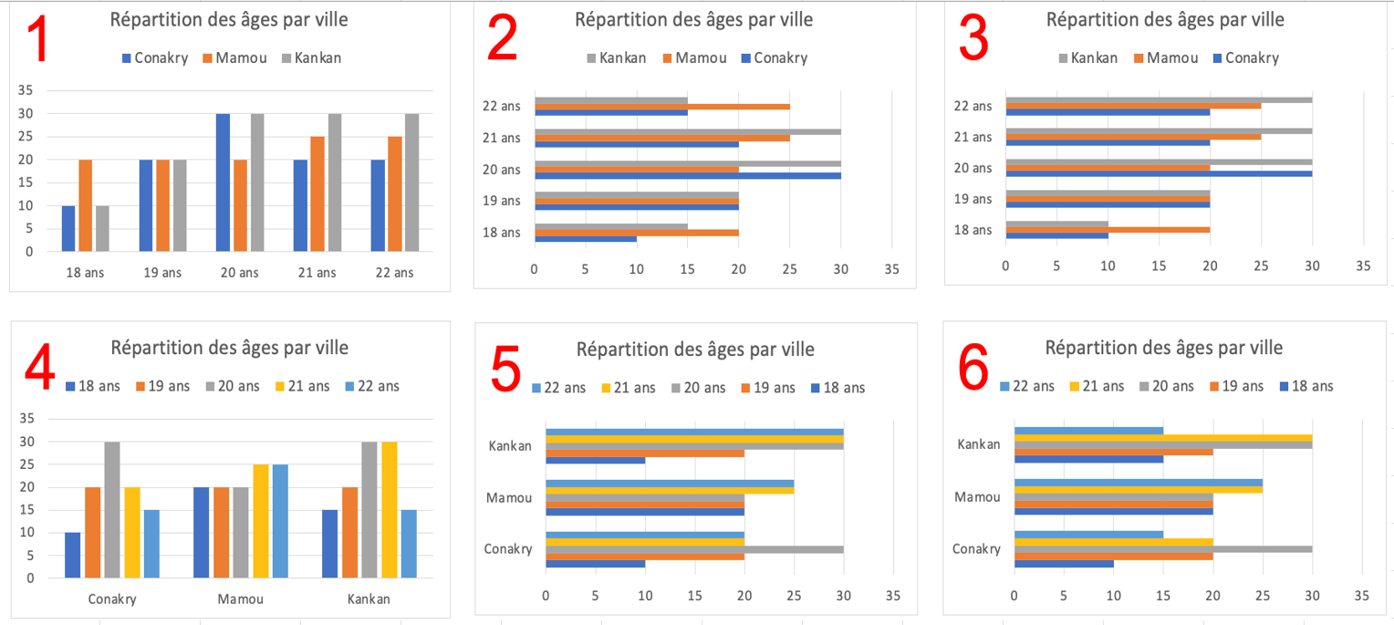
- Copy the result into your report and indicate the number of the chart obtained among the six charts shown below.
- Copier le résultat dans votre compte rendu et préciser le numéro du graphe obtenu parmi les 6 graphes ci-dessous:

- Data Sorting
This section covers formatting using Data Sorting.
Tris de données
Cette partie aborde la mise en forme avec Tri des données:
- Question 3.6
Open the spreadsheet page, click here:
Ouvrir la page de travail, cliquer-ici:
Відкрийте робочу сторінку, натисніть тут:
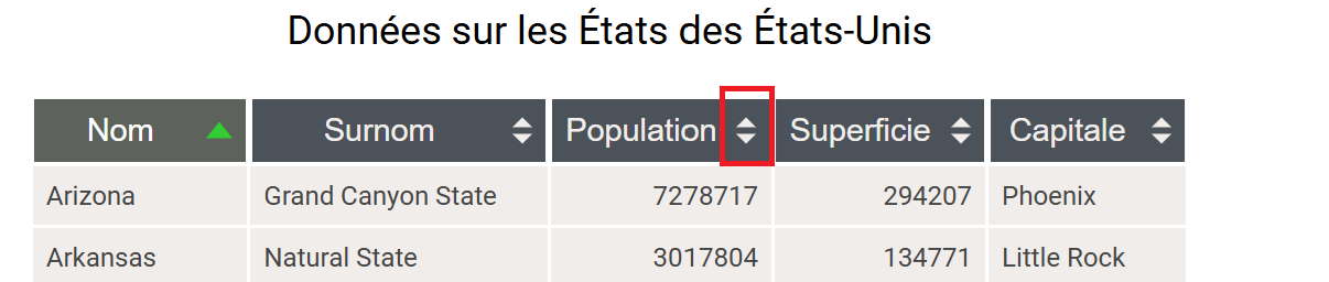
Sort this table so that the state with the largest population appears first. In the sorted table, what is the capital of the 4th state?
Triez ce tableau pour afficher en premier, l'état avec la plus grande population. Dans le tableau trié, quel est la capitale du 4eme état ?

To answer this question, follow the steps below:
- Sort the Population column as requested in the question by clicking on the arrows (circled in red below).
Pour répondre à cette question, suivre la démarche ci-dessous:
- Ranger la colonne Population comme demandée dans la question en cliquant sur les flèches ( entourées en rouge ci-dessous):

- Write down in your report the capital of the 4th state.
- Noter sur votre compte rendu la capitale du 4eme état
- Question 3.7
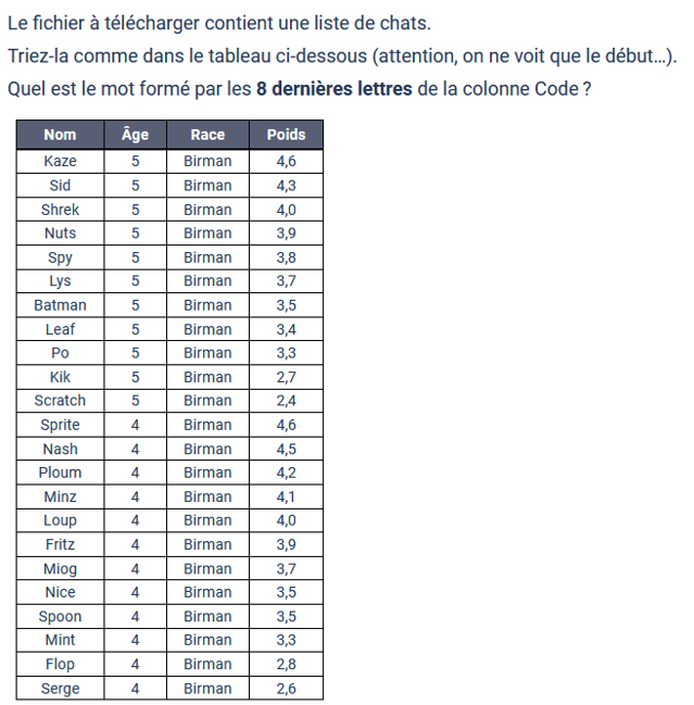
The file to download contains a list of cats.
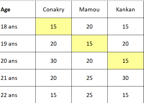
Sort it as shown in the table below (note: only the beginning is visible...).
What word is formed by the last 8 letters of the Code column?

- Open the cats file (click here)
- Ouvrir le fichier chats ( cliquez-ici)
Method to follow:
- Select the entire table
Click on a cell in the table, then use the keyboard shortcut Ctrl + A to select everything.
Méthode à suivre:
1. Sélectionner tout ton tableau
Cliquer sur une cellule du tableau, puis utiliser les touches du clavier Ctrl + A pour tout sélectionner .
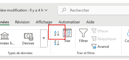
2. Go to the Data tab in the top ribbon.
Aller dans l’onglet Données du ruban supérieur.

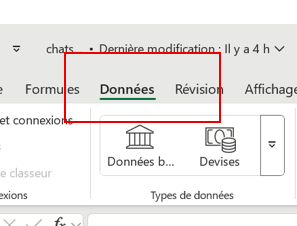
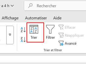
3. Click Sort using the Advanced Sort icon (outlined in red below).
Cliquer sur Trier avec l’icône de tri Avancé ( encadrée en rouge ci-dessous).
4. Add two sorting levels by clicking + Add Level.
Ajouter deux niveaux de tri en cliquant sur +Ajouter un niveau:
Avant: Après:
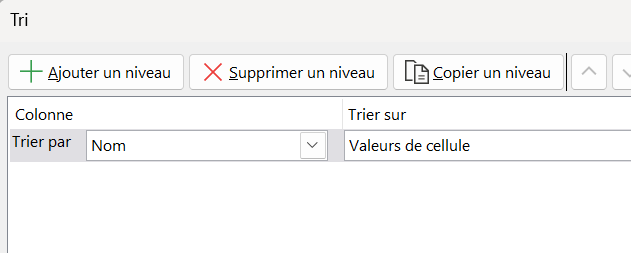
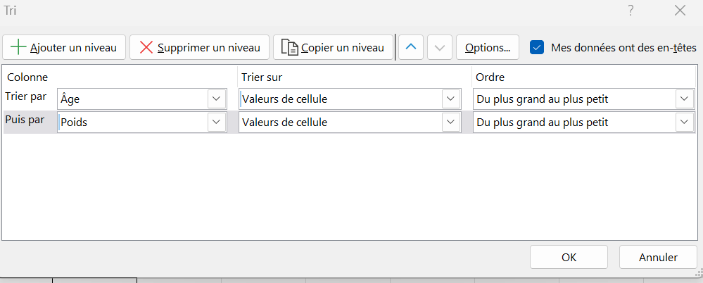
In the Sort dialog box, configure:
First level:
Sort by: Age
Order: Descending (from largest to smallest)
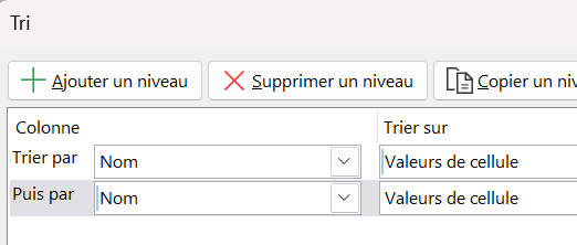
Second level:
Then by: Weight
Order: Descending (from largest to smallest)
Dans la boîte de dialogue de Tri, configurer:
- Premier niveau :
- Trier par : Âge
- Ordre : Décroissant (du plus grand au plus petit)
- Deuxième niveau :
- Puis par : Poids
- Ordre : Décroissant (du plus grand au plus petit)

5. Confirm by clicking OK
Valider avec OK
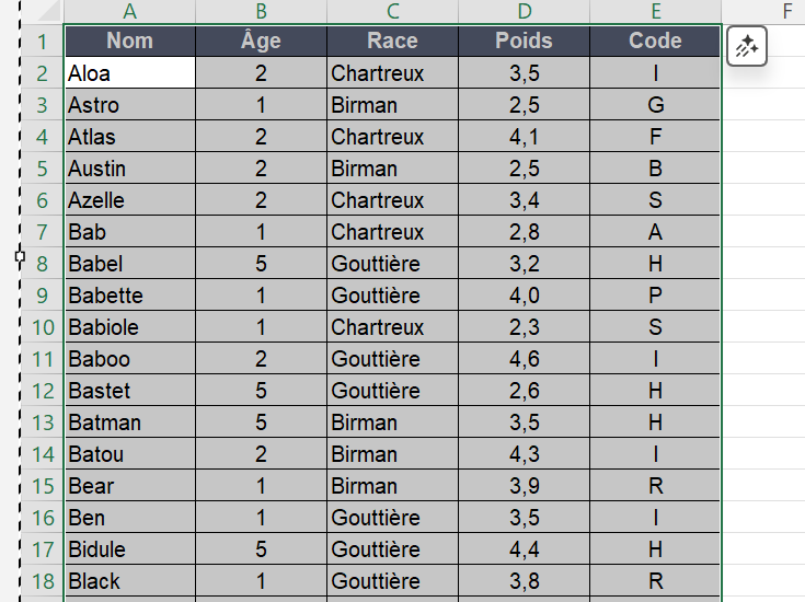
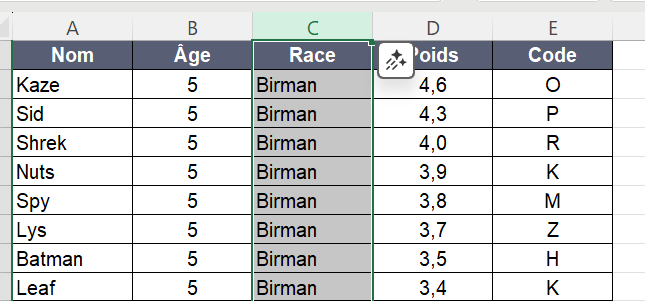
6. Click on the C of the Race column to select it, then click the Sort A to Z button (shown in red below). The cat breeds will now start with Birman and will be sorted by age and weight.
Cliquer sur le C de la colonne Race pour la sélectionner puis sur le bouton trier de A à Z ( en rouge ci-dessous), la race des chats commencent par Birman et sont classés par âge et poids:
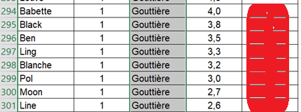
7. Go to the bottom of the page using the scroll bar, identify the word in the Code column from Babette to Line, and write it down in your report.
Se rendre en bas de la page avec la barre de défilement et relever le mot de la colonne Code à partir de Babette jusqu'à Line et le noter dans votre compte rendu:

Créé avec HelpNDoc Personal Edition: Générer facilement des livres électroniques Kindle